Demystifying Artificial Neural Networks, Part 2

In this blog I thought I’d give you a bit of an idea about how Feed Forward Artificial Neural Networks work. As you might imagine, this is a huge topic and this blog became tl;dr before I really knew it, so try to hang in there and give me feedback (if you like) on what you read here.

And BTW, if you know a good way to write math in wordpress please let me know.

Thanks, and safe and happy holidays to you and your families.

–dmm

So What is Machine Learning Anyway?

While there are several formal models of what Machine Learning (ML) is or does, whenever I’m asked what machine learning is all about, this quote from Andrew Ng  is always the first thing that comes to mind:

The complexity in traditional computer programming is in the code (programs that people write). In machine learning, algorithms (programs) are in principle simple and the complexity (structure) is in the data. Is there a way that we can automatically learn that structure?  That is what is at the heart of machine learning.

That is, ML is the about the construction and study  of systems that can learn from data. What exactly does this mean? Basically ML is about building statistical models from training data that can be used to predict the future, usually by either classification or by computing a function.  This is a very different paradigm than we find in traditional programming. The difference is depicted in cartoon form in Figure 1.

Figure 1: Traditional Programming vs. Machine Learning

So basically we want to build models that, when given some prior information (which may not only be training data but also knowledge of priors), can generalize to predict

• The probability of a yes/no event
  • e.g. customer likes product, image contains a face, …
• The probability of belonging to a category
  • e.g. emotion in face image: anger, fear, surprise, happiness, or  sadness, …
• The expected value of a  continuous variable
  • e.g. expected game score, time to next game, …
• The probability density of a  continuous variable
  • e.g. probability of any interval of values, …
• And many others…

Basic Assumption: Smoothness

So what assumptions do we need to be able to predict the future?  That is, what are the key assumptions that allow us to build generalizable statistical models from input data? To get a qualitative idea of what is required,  consider what it takes to learn the function f(x) depicted in Figure 2.

Figure 2: Easy Learning (courtesy Yoshua Bengio)

In this case  learning f(x) is relatively easy because the training data closely models the true (but unknown) function, that is, the training data that hits most of the ups and downs in the function to be learned.  The basic property of these easy cases (e.g., Figure 2) that allows the learned model to generalizes is that for a training example x and a test input x’, if x is geometrically close to x’, then we assume that  f(x) ≈ f(x’). Clearly this is true for the function and data depicted in Figure 2.

The assumption that f(x) ≈ f(x’) when x is close to x’ is called the Smoothness Assumption, and it is core to our ability to build generalizable models. The Smoothness Assumption is depicted for a simple quadratic  function  in Figure 3.

Figure 3: Smoothness Assumption — x geometrically close to x’  → f(x) ≈ f(x’)

Well, that is all cool except that the functions we want to learn in ML are nothing like the functions depicted in Figures 2 or 3.  Instead, real data from functions we want to learn are typically concentrated near highly curved (potentially high dimension) sub-manifolds, as shown in Figure 4. This concentration is sometimes called “probability mass”, since the probability of finding representatives of the class we’re trying to learn will in general be higher near the surface where the data are concentrated.

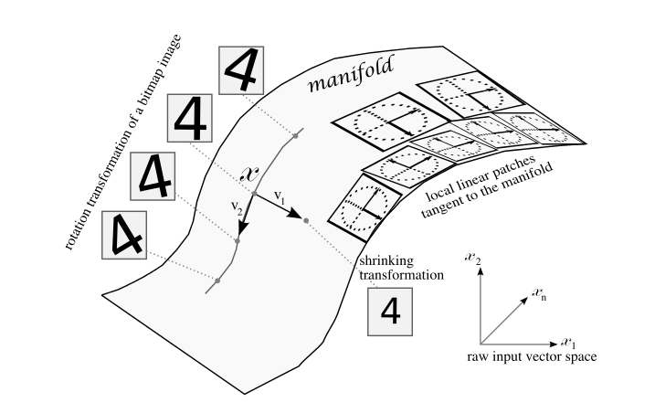
Figure 4: Sub-manifold for the handwritten digit 4

Notice that the manifold in Figure 4 is something of an “invariance” manifold. That is, images on the  manifold (in this case the handwritten digit 4) are in theory invariant to translation and rotation. We need this invariance property, because after all, I want to be able to recognize a face (or whatever) even in the presence of say, out of plane rotation, so we need a representation that accommodates this kind of translation. So we assume that things that are alike concentrate on a manifold as shown in Figure 4 (note that this is just a higher dimensioned generalization of what is shown in Figure 3).

Incidently, rotational/translational invariance of the kind shown in Figure 4 is precisely what breaks down in the presence of the custom crafted adversarial images discussed in Intriguing properties of neural networks?.   These studies show that under certain conditions an adversarial image can “jump off” the manifold and as a result won’t be recognized by a learner trained to build such an invariance manifold. Other studies have shown the converse: adversarial images can constructed (in the case cited, with evolutionary algorithms) that fool the trained network into misclassifying what is essentially white noise.

Before moving on, I’ll just note here that deep learning has emerged as a promising technique to learn useful hidden representations (such representations that residmust generalize well. e on manifolds as described above) which previously required hand-crafted preprocessing; we’ll  talk about what hidden means below.  This input preprocessing essentially came down to using a human to tell the learning algorithm what the important features were; the SIFT algorithm is a canonical example from the field of computer vision. What SIFT does is preprocess the input data so that the machine learning step(s) will be more efficient.  I’ll note here that prior to the success of unsupervised deep learning systems in discovering sailent features, most of the effort in building say, a machine learning system to recognize faces, was in the crafting of features. Modern machine learning techniques seek to remove humans from the feature crafting/discovery loop. We’ll take a closer look at deep learning and its application to representation learning in upcoming blogs.

When might we use Machine Learning?

Machine learning is most effective in the following situations:

• When patterns exists in our data
  • Even if we don’t know what they are
  • Or perhaps especially when we don’t know what they are
• We can not pin down the functional relationships mathematically
  • Else we would just code up the algorithm
  • This is typically the cases for image or sensor data, among others
• When we have lots of (unlabelled) data
  • Labelled training sets harder to come by
    • Labelled data has a tag that tells you what it is, e.g., this is a cat
    • Most data isn’t labelled
• Data is of high-dimension
  • Dimensionality of input data is a problem that all machine learning approaches need to deal with. For example,  we’re looking at 1Kx1K grey scale images, the input has 1048576 dimensions in pixel space. This high dimensionality leads to what is know as the curse of dimensionality;  basically as the dimensionality of the input data increases, the volume of the input space increases exponentially, so the available data become sparse, and sparse input poses interesting problems for statistical (and other) methods. This also means we are unlikely to see examples from most regions of the input space, so in order to be effective a model or set of models must generalize well (noting that  model averaging is a powerful technique to minimize prediction error). he curse of dimensionality problem is depicted in Figure 5.
    • BTW, how do we learn to recognize images in nature?  Well, consider the space of images that we humans can see. These images have something like 10^6×10^6 or 10^12 dimensions in pixel space  (yes, your eyes are perceiving input in more than a trillion dimensional space);  this number comes from the fact that there are on the order of 10^6 fibers in the optic nerve running from each of your retinas to your visual cortex.  Given that the distribution of cones and rods in the average human retina has a maximum of something like (1.5 x 10^5)/mm^2 in the average human retina, we can make a conservative guess and say we have 256 bits to represent color at each point (we’re clearly under-estimating the number of colors/shadings we can perceive;  color vision in mammals is of course more complex than this, with fascinating theories going back to Newton and Maxwell). But even without looking at color (or gray scale, or …), using this simplifying assumption gives us a  conservative estimate of the size of the trillion dimensional image space to be  something like 2^(10^12) , an enormous and computationally intractable number. Given this huge space and the computational challenges it implies, how is that we learn to recognize any image at all?  The answer is that we can learn the images we encounter in nature because that set is much, much smaller than the size of the total image space. That is, the set of naturally occurring images is sparse.  
  • Sensor, audio, video, and network data, to name a few, are all high dimension
• Want to “discover” lower-dimension (more abstract) representations
  •  Several dimension-reduction techniques are used in machine learning (e.g., Principal Component Analysis, or PCA) and we will discuss these in later blogs but as a hint, the basic idea behind techniques like PCA is to find the important aspects of the training data and project them onto a lower dimension space.
• Aside: Machine Learning is heavily focused on implementability
  • Frequently using well know numerical optimization techniques
  • Heavy use of GPU technology
  • Lots of open source code available
    • See e.g., libsvm (Support Vector Machines)
    • Most of my code these days is in python (lots of choices here)

Figure 5: The Curse of Dimensionality — at high dimension data becomes sparse

As we can see from the discussion above, machine learning is primarily about building models that will allow us to efficiently predict the future. What does this mean? Basically its a statement about how well a particular model generalizes.  

But what does generalizing really mean? We can characterize a model that generalizes as one that captures the dependencies between random variables while spreading out the probability mass from the empirical distribution (homework: why is this part of generalization?). At the end of the day, however, what we really want to do is to discover the underlying abstractions and explanatory factors which make a learner understand what is important (and frequently hidden) about the input data set. No small task.  Two of the key problems encountered when trying to build generalizable models are overfitting and underfitting (the evil twins of  bias and variance) which I’m not going to talk about here here other than to say that there are also basic statistical barriers that make model generalization tricky; I’ll leave that for a future blog.

Examples of Machine Learning Problems

Machine learning is a very general method for solving a wide variety of problems, including

• Pattern Recognition
  • Facial identies  or facial expressions
  • Handwritten or spoken words (e.g., Siri)
  • Medical images
  • Sensor Data/IoT
  • …
• Optimization
  •  Many parameters have “hidden” relationships that can be the basis of optimization
• Pattern Generation
  • Generating images or motion sequences
• Anomaly Detection
  •  Unusual patterns in the telemetry from physical and/or virtual plants
    • For example, data centers
  • Unusual sequences of credit card transactions
  • Unusual patterns of sensor data from a nuclear power plant
  • or unusual sounds in your car engine or …
• Prediction
  •  Future stock prices or currency exchange rates

Types of Machine Learning

Supervised Learning

The main types of machine learning include Supervised Learning, in which the training data includes desired outputs (i.e., supervised learning requires “labelled” data sets).  All kinds of “standard” (benchmark)  training data sets are available, including  http://archive.ics.uci.edu/ml/ (UCI Machine Learning Repository), http://yann.lecun.com/exdb/mnist/ (subset of the MNIST database of handwricen digits), and http://deeplearning.net/datasets/, to name a few.

Unsupervised learning

In Unsupervised Learning, the training data does not include desired outputs. This is called “unlabelled data” (for obvious reasons). Most data is of this type, and new techniques such auto-encoders have been developed to take advantage of the vast amount of unlabelled data that is available (consider the number of video frames available on youtube, for example).

Other Learning Types

There are many other learning types that have been explored. Two of the most popular are Semi-supervised Learning, in which the training data includes a few desired outputs (some of the training data is labelled, but not all), and Reinforcement Learning, in which the learner is given rewards for certain sequences of actions.

Artificial Neural Networks (ANNs)

Before diving into ANNs, I’ll just point out that you can think of an ANN is a learning algorithm that learns a program from its training data set(s). How does it learn? See below. That said, there are various kinds of learning that broadly fall into supervised, semi-supervised, and unsupervised classes.  There are a daunting number of learning algorithms created every year, but the ANN remains one of the most interesting as well as being one of the most successful on various tasks. And as we will see below, you can think of the weights and biases that an ANN learns as a program that runs on the ANN. In this blog we will consider only Feed Forward ANNs. Feed Forward ANNs  form directed acyclic graphs (DAGs), whereas in Recurrent Neural Networks (RNNs)  the connections between units are allowed to form directed cycles. This allows RNNs to model memory and time in ways that a Feed Forward ANN can not. See such as Long Short Term Memory (LSTM) networks for an interesting RNN.

As described in an earlier blog, an ANN is comprised of Artificial Neurons which are arranged in input, hidden, and output layers. Figure 6 reviews the structure and computational aspects of an Artificial Neuron and compares it to its biological counterpart.

Figure 6: Biological and Artificial Neurons

As described in Demystifying Artificial Neural Networks, Part 1, a single artificial neuron (AN) can compute functions with a linear decision boundary. The intuition here is that if you can draw a straight line separating the values of the function that the AN is trying to compute, then that function is said to be linearly separable and is computable by a single AN. This is depicted in Figure 7.

Figure 7: OR and AND are linearly separable

On the other hand, functions such as XOR are not linearly separable, since a straight line can not be drawn that separates the values of the XOR function (this result generalizes to a hyper-plane in higher dimensional spaces).  This is shown in Figure 8.  Note however that we may be able to transform the input into something that is linearly separable with another layer of ANs as shown in the right side of Figure 8.

Figure 8: XOR is not linearly separable

A single hidden layer  ANN is depicted in Figure 9. The hidden layer is called hidden because it is neither input nor output, and its representation of the salient features of the input are not “seen”. From this example we might guess that if we have more layers in our ANN we can compute progressively more complex functions.  So maybe the “deeper” the network (more layers), the more we can compute? It turns out that this intuition is for the most part correct.

Figure 9: Single Hidden Layer ANN

So we saw that a single AN can compute functions that are linearly separable. What about ANN’s with a single hidden layer? Well, it turns out that there is an Universal Approximation Theorem which states that “a single hidden layer neural network a linear output unit can approximate any continuous function arbitrarily well, given enough hidden units”.  Well, that’s cool. The problem is that the single layer ANN may need exponentially many hidden units, and and there is no guarantee that a learning algorithm can find the necessary parameters.

Feed Forward Neural Networks

The computation of the activation of a single AN is shown in Figure 10. The activation (or output) of the neuron, ,  is the linear sum of the weights  times the input values  plus a bias term b.  Frequently a “pre-activation”, usually denoted as a(x),  is useful to compute as an intermediate result, where .

A cartoon of the basic forward propagation in a Feed Forward Neural Network is shown in Figure 11. The basic idea is that you calculate the output of each neuron at each layer, starting with layer 1 (the input to layer 2 are the outputs from layer 1, etc), and propagate those results forward through the network to the output layer, which is why its called a feed-forward network.

More formally, we see that the output of a single AN is   or just  .   is called the hypothesis (for historical reasons), and is parametrized by θ, the set of weights and biases that have been learned so far.  This is called the feed forward activation of the AN (you might wonder where the ‘s  and the b‘s come from…more on that in a minute).  Popular choices for the activation function g are shown in Figure 12.

Figure 10: Artificial Neuron Computation (graphic courtesy Hugo Larochelle)

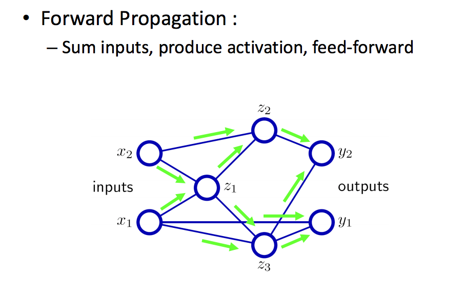
Figure 11: Feed Forward Processing

I’ll just note here that popular ANNs use non-linear activation functions such as the logistic or hyperbolic tangent activation functions. A notable exception is the Google deep auto-encoder, which uses a linear activation function. In addition, the Rectified Linear Unit (ReLU) has recently become a popular activation function; this is interesting because the ReLU doesn’t have a smooth derivative (or a derivative at all in some regions), which will make the optimization problem described below a bit harder. The general form of the ReLU function is . Kind of amazingly, the derivative of the ReLU function is , which is just the logistic function shown in Figure 12. Interesting…

Figure 12: Popular Activation Functions

So how do we compute the feed forward output of a more complex ANN? The feed forward computation for a single hidden layer single output function ANN is shown in Figure 13.

Figure 13 Single Hidden Layer ANN Feed Forward Computation

As you can see from Figure 13, we calculate the activations for the (single) hidden layer in the say way we did the single AN, namely, for a hidden unit  i in layer 1 (the single hidden layer), the activation of any neuron is simply . We can generalize this to L hidden layers, as shown in Figure 14. In general, the higher hidden layers of an ANN compute successively more abstract representations of the input data.

Figure 14: L-Layer Feed Forward Neural Network

The final piece of the feed forward computation is the output  function. In Figure 14, the output layer is layer 4, or the top layer of the ANN.  While the computation works in the same way. Suppose we have L hidden layers.  Then by convention the input layer is called layer 0 and hence the output layer is layer L+1. The input to each output unity i  is  and a unit i in the output layer is  .  The output function o  varies depending what what we’re trying to accomplish. For example, if we’re building an n-way classifier, we might use the softmax function as the output function o.

 Ok, But Where Do the Weights and Biases Come From?

Learning in ANNs comes down to learning the weights and biases (this is a form of Hebbian Learning, which is named after Canadian psychologist Donald Hebb). So for our purposes, the application of the Hebbian principle at work is that learning consists of adjusting weights and biases.  So how are the weights and biases learned?

Overview of the Learning Process

I suspect that this blog is already a tl;dr, so I’m just going to overview how training works and I’ll leave the details (there are many) for the next blog. So we know how, given an ANN, how to calculate the feed forward output    of the ANN for a given set θ of weights  and biases .  Figure 15 reviews the feed-forward stage for an ANN. 

 

Figure 15: Feed-Forward Calculation

How might you code up the feed forward step in python? Figure 16 shows how to do it with pybrain. These days I tend to use pylearn2 but there are lots of choices. Others include scikit-learn, theano, weka (if you like java), and many more. There are also quite a few languages that are primarily  built for numerical computation (and as such have key functions built in) such as octave.  You can also write code in octave since it has its own language.

Figure 16: Build and activate a Feed Forward ANN in pybrain

For this discussion, assume we are using supervised learning (we’ll talk about the unsupervised case in the next blog).  In practice this means that for each input   we also know the label .  The ‘s will typically be something like “this is a cat”,  “this is a motorcycle”, etc.

Estimating The Loss (or Cost, Error) of Our Prediction

Now that we know how to calculate   and we are given , we can get some intuition about what kind of error or loss that the current value of θ produces for each .  As a first approximation, a reasonable guess for current error might be  something like  or maybe  (the standard squared error).  So a candidate loss function might look  something like  ; this is a typical loss function for linear regression (note that convention is to use a bold font to indicate that you are  talking about a vector and subscript when you’re talking about an element of the vector). BTW, construction of loss functions are a big part of building a machine learning system.  I’ll just note here that loss functions are also called cost functions and are sometimes denoted J(θ).

Given our loss function , a simple learning algorithm might look something like:

1. Initialize the parameters θ to random values
2. Foreach  in our training set  
   1. Calculate                                                       # forward propagation step
   2. Calculate the loss function 
   3. Adjust θ so that our error   is minimized 
3. End

We might consider this to be “learning”.  Kinda makes sense. We want the error of our prediction to be minimized. So here is the important leap:

Learning is, among other things,  an optimization problem

More generally,  learning algorithms that try to minimize the error (loss) such as described in the pseudo-code above are instances of Empirical Risk Minimization (ERM). What ERM tries to do is to find the values of θ that minimize the values of the loss function on the training data set. Basically what we want to do is find the weights and biases that minimize our prediction error. In the algorithm described above,   can be minimized using the back propagation algorithm. Backpropagation is an abbreviation for the “backward propagation of errors”, and is a common method of training artificial neural networks that is used in conjunction with an optimization method such as gradient descent.  The method calculates the gradient of a loss function with respects to all the weights in the network (hint: a gradient is just a fancy word for the generalization of the usual concept of derivative of a function in one dimension to a function in several dimensions). The gradient is fed to the optimization method which in turn uses it to update the weights θ in an attempt to minimize the loss function. As we’ll see below, there are ways for this to go wrong, such getting caught in a local minima when the function being optimized is non-convex.

Solving this optimization problem is one of the major challenges for machine learning (along with choosing a good representation and finding an effective objective/loss function), and there are many techniques that yield good results in a variety of learning setting.  And of course, these problems are typically NP-hard so exact solutions aren’t going to be feasible in most cases. As a result, many of the problems that we want solve with machine learning do not have known analytic solutions for the optimization problem (in fact, only the “easy” problems such as linear regression have closed forms).  Consequently most machine learning optimization problems are solved with a numerical method such as Stochastic Gradient Descent, L-BFGS, or Newton’s method.

Just one more quick comment on all of this: how many parameters (θ) are being learned in a state of the art machine learning system? Another way to ask this is to ask what is the size of the optimization problem that these systems are solving?  Literally billions, which gives you some idea of what kind of computational resources are required and why GPUs are so popular with folks who implement machine learning systems.

Brief Aside On Optimization

Solving large sometimes non-convex optimization problems is a key challenge for machine learning. Why is non-convex optimization hard?  There are many reasons but  let’s look at one obvious feature of convex vs. non-convex optimization. First, a technique like gradient descent essentially follows the gradient “down”, looking for the minimum value; makes sense, if the “slope” is pointing down, maybe that is the direction of the minimum. So in the case of a convex function such as the one depicted in Figure 17, this works perfectly. As you can see, for a convex function any local minima is also a global minimum, a very nice feature indeed. The bottom line here is that if you are trying to minimize a convex objective function, you can start anywhere and get to the global minimum.

 

Figure 17: Convex Loss Function

Unfortunately, almost any interesting loss function we might want to use for machine learning will be non-convex. A typical non-convex “landscape” is shown in Figure 18.

Figure 18: Non-Convex Loss Function

As you can see from Figure 18,  if you start in the “wrong” place, you might follow the gradient down into a local minima which is not the global minimum. In other words, the optimization procedure can get stuck in a local minima, since in such a minima everywhere you “look” the gradient points upward and as a result you think you’re at the bottom (but you aren’t) and you’re stuck.  So in the case of non-convex loss functions, the optimization procedure will be sensitive to the initial settings of θ, suggesting that random initialization might not be a sensible way to initialize θ.

Given that this is tl;dr already, we’ll talk about methods for solving the optimization problem in the next blog (so dust off your vector calculus and brush up on gradients and Hessian matrices).